Table Of Content
However, your data isn't in a true "table" unless you've used the specific Excel data table feature. To select the table data area, click the upper-left corner of the table, the mouse pointer will change to a south-east pointing arrow like in the screenshot below. To select the entire table, including the table headers and total row, click the arrow twice.
Excel Tutorial: Where Is Table Design In Excel
Then, check the Total Row box in the Table Style Options group. Once the Total Row is added, you can select the desired column and choose the function from the drop-down list to display the result in the Total Row. Tables have a feature called calculated columns that makes entering and maintaining formulas easier and more accurate. When you enter a standard formula in a column, the formula is automatically copied throughout the column, with no need for copy and paste.
Creating Custom Table Style
If you want to use it in another workbook, the fastest way is to copy the table with the custom style to that workbook. You can delete the copied table later and the custom style will remain in the Table Styles gallery. To delete a custom table style, right-click on it, and select Delete.
Adding and removing table headers
Microsoft Designer: Get inspired with new AI features - Microsoft
Microsoft Designer: Get inspired with new AI features.
Posted: Thu, 27 Apr 2023 07:00:00 GMT [source]
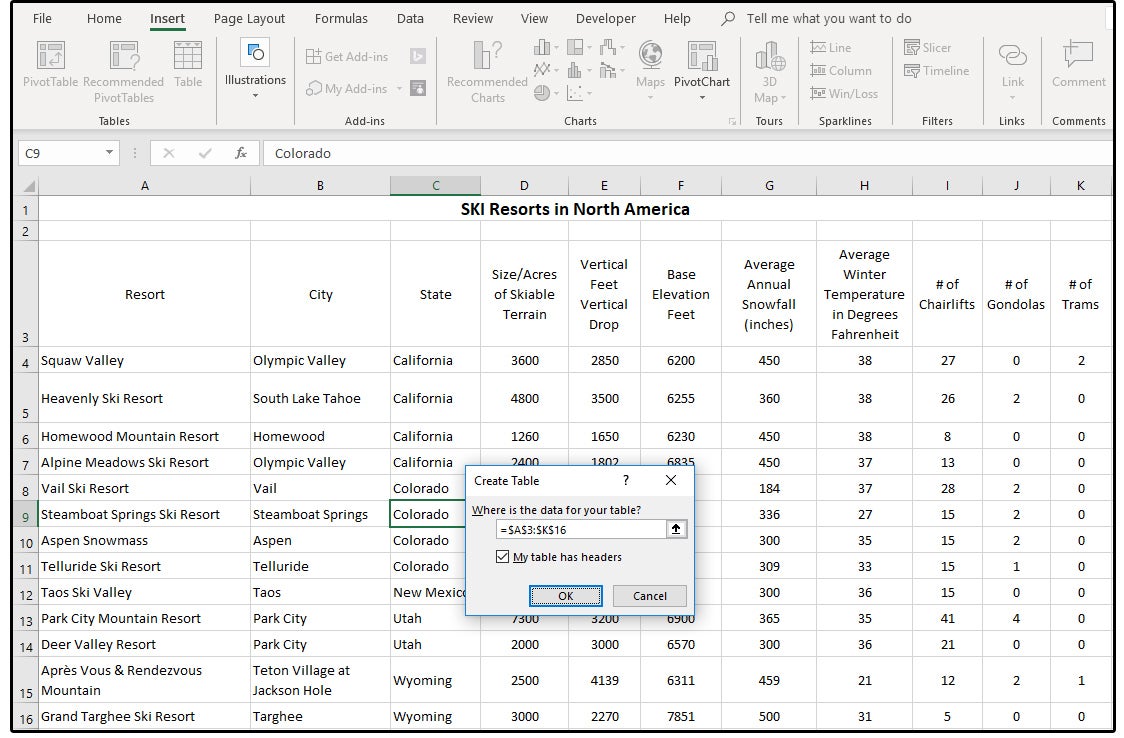
Table names are a must when you create large, robust Excel workbooks. It's a housekeeping step that ensures you know where your cell references point to. Start off by clicking inside a set of data in your spreadsheet. You can click anywhere in a set of data before converting it to a table. To follow along with this tutorial, you can use the sample data I've included for free in this tutorial. It's a simple spreadsheet with example data you can use to convert to a table in Excel.
How To Make a Table in Excel Quickly (Watch & Learn)
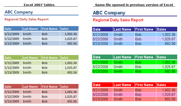
Impress your prospects with a unique and memorable table design enriched with many colors, icons, fonts, and styles to choose from. We create short videos, and clear examples of formulas, functions, pivot tables, conditional formatting, and charts. All Excel tables have a style applied by default, but you can change this at any time.
Business Central & Excel: Viewing & Editing Features - FORVIS
Business Central & Excel: Viewing & Editing Features.
Posted: Mon, 20 Feb 2023 08:00:00 GMT [source]
How to Create an Effective Excel Dashboard
Excel provides a variety of table functions to help users analyze and summarize data within a table. In this chapter, we will explore the basics of using table functions and how to create custom functions for specific data analysis needs. Table design is an essential aspect of Excel that can greatly improve the functionality and appearance of your data. Whether you're organizing information, creating reports, or analyzing data, a well-designed table can make your work more efficient and visually appealing. In this Excel tutorial, we will take a brief overview of where to find table design features in Excel so you can elevate your data presentation and analysis skills. Tables make it much easier to rearrange data with drag and drop.
The Count function can be used to count the number of entries in a column, providing valuable insights into the data. Table functions in Excel are powerful tools that allow users to perform calculations and analysis within a table of data. The most commonly used table functions include Total, Average, and Count.
This will add your data to a table and then open the Power Query Editor where you will be able to build your query based on the new table. Power Query is a very useful tool for transforming your data, but you can also create a table during the process of building your queries. This should automatically show the Quick Analysis tool in the lower right corner of the selected range. There is also a legacy shortcut available from when tables were called lists. Select your data and if you press Ctrl + L this will also make a table.
Create your own Tables with World’s Best Online Table Generator
When new rows or columns are added to an Excel Table, the table expands to enclose them. In a similar way, a table automatically contracts when rows or columns are deleted. When combined with structured references (see below) this gives you a dynamic range to use with formulas.
This will delete a table but keep all data and formats intact. Excel will also take care of the table formulas and change the structured references to normal cell references. When you create a chart based on a table, the chart updates automatically as you edit the table data. Once a new row or column is added to the table, the graph dynamically expands to take the new data in. When you delete some data in the table, Excel removes it from the chart straight away.
To remove table headers, simply deselect the "Header Row" checkbox. When working in Excel, it's important to be able to modify the properties of your tables to best fit your data and presentation needs. This can include changing the size and layout of the table, as well as adding or removing table rows and columns.
As we have seen, slicers are a powerful tool for enhancing the functionality of Excel tables and simplifying the data analysis process. By utilizing slicers effectively, users can gain valuable insights from their data in a more efficient and intuitive manner. Slicers work by enabling users to easily filter and analyze data by selecting from a list of options. When a slicer is connected to a table, it allows users to filter the data by simply clicking on the desired option. In this section, we will explore how slicers can be used to enhance the functionality of Excel tables and make data analysis easier and more efficient.
Select any cell in the table and use the Table Styles menu on the Table Tools tab of the ribbon. The Total Row can be easily configured to perform operations like SUM and COUNT without entering a formula. When the table is filtered, these totals will automatically calculate on visible rows only. You can toggle the Total Row on and off with the shortcut control + shift + T.
The column headings are added to each new sheet starting in cell A1. You can adjust the above line of code to change the column headings to suit your needs. If you are using Excel online and want to automate the process of creating multiple tables from a list, then you will need to use Office Scripts. The above line of code is used to create the column headings in each table. This is a great option as you get to choose the table style during the process of making your table.
By following these steps, you can easily sort and filter data in Excel tables to efficiently analyze and work with your data. Filtering data in Excel tables allows you to display only the rows that meet specific criteria, making it easier to analyze and work with the data. By removing only the formatting, such as banded rows, shading, and borders, you may maintain all the features of an Excel table. Best of all, if the table changes with new rows or columns, these references are smart enough to update as well.


No comments:
Post a Comment